A linear differential equation is a differential equation in which the function and its derivatives appear only to the first power and, thus, are not multiplied or divided by each other.
General Form
A nth order linear differential equation is an equation of the form:
${a_{n}\left( x\right) \dfrac{d^{n}y}{dx^{n}}+a_{n-1}\left( x\right) \dfrac{d^{n-1}y}{dx^{n-1}}+\ldots +a_{1}\left( x\right) \dfrac{dy}{dx}+a_{0}\left( x\right) y=g\left( x\right)}$
Here,
- y is the dependent variable
- x is the independent variable
- a0(x), a1(x), …, an(x) are functions of x
- g(x) is a given function (forcing function)
The above general form is linear because y and its derivatives have exponent 1.
Types
All linear differential equations (first, second, or higher orders) can be either homogeneous or non-homogeneous. If the function g(x) on the right-hand side is zero, the equation is called homogeneous, or it is non-homogeneous.
First-Order
A first-order linear differential equation has the form:
${\dfrac{dy}{dx}+P\left( x\right) y=Q\left( x\right)}$
Here,
- P(x) and Q(x) both are continuous functions of x
Here are a few examples of first-order linear differential equations:
${\dfrac{dy}{dx}-3y=x}$
${\dfrac{dy}{dx}+5y=\cos x}$
Solving
One common method for solving first-order linear differential equations is the Integrating Factor Method. Here, we will determine a function of the independent variable, which is known as the Integrating factor (I.F).
The differential equation ${\dfrac{dy}{dx}+P\left( x\right) y=Q\left( x\right)}$ has the integrating factor I(x), which is:
I(x) = ${e^{\int Pdx}}$
${\dfrac{dy}{dx}+P\left( x\right) y=Q\left( x\right)}$
Multiplying the equation by the integrating factor,
⇒ ${e^{\int Pdx}\dfrac{dy}{dx}+Pe^{\int Pdx}y=Qe^{\int Pdx}}$
Here, we observe that the left-hand side is the derivative of yI(x).
⇒ ${\dfrac{d}{dx}\left( ye^{\int Pdx}\right) =Qe^{\int Pdx}}$
Now, integrating both sides with respect to x, we get
⇒ ${ye^{\int Pdx}=\int Qe^{\int Pdx}dx+C}$
Solving for y,
⇒ ${y=\dfrac{1}{e^{\int Pdx}}\left( \int Qe^{\int Pdx}dx+C\right)}$
Here, C is some integrating constant.
Let us consider an example to understand the concept better.
Problem: Solving linear differential equation by the INTEGRATING FACTOR METHOD
![]() Solve: ${\dfrac{dy}{dx}+2y=e^{-x}}$
Solve: ${\dfrac{dy}{dx}+2y=e^{-x}}$
Solution:
Solving this equation by the Integrating Factor Method, we get
Given, ${\dfrac{dy}{dx}+2y=e^{-x}}$ …..(i)
Step 1: Identifying P(x) and Q(x)
Here, P(x) = 2 and Q(x) = e-x
Step 2: Calculating the Integrating Factor
The integrating factor is I(x) = ${e^{\int 2dx}}$ = e2x
Step 3: Multiplying the Equation by I(x)
${e^{2x}\dfrac{dy}{dx}+2e^{2x}y=e^{2x}e^{-x}}$
⇒ ${e^{2x}\dfrac{dy}{dx}+2e^{2x}y=e^{x}}$
Step 4: Rewriting in a Recognizable Form
⇒ ${\dfrac{d}{dx}\left( ye^{2x}\right) =e^{x}}$
Step 5: Integrating Both Sides
⇒ ${ye^{2x}=\int e^{x}dx}$
⇒ ye2x = ex + C
Step 6: Solving for y
⇒ y = e-2x(ex + C)
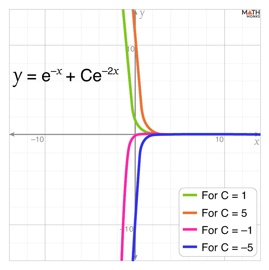
⇒ y = e-x + Ce-2x, which is the general solution.
The graph to the right shows the solution of ${\dfrac{dy}{dx}+2y=e^{-x}}$. The solution y = e-x + Ce-2x varies depending on the integration constant C.
Second-Order
A second-order linear differential equation takes the form:
${\dfrac{d^{2}y}{dx^{2}}+a\dfrac{dy}{dx}+by=g\left( x\right)}$
Here are a few examples of first-order linear differential equations:
${\dfrac{d^{2}y}{dx^{2}}-3y=x^{2}}$
${\dfrac{d^{2}y}{dx^{2}}+\dfrac{dy}{dx}+y=5x}$
To solve higher-order differential equations, we divide them into two main cases:
Solving
Second-order linear differential equations can be solved by different methods depending on whether the equations are either homogeneous or non-homogeneous.
Problem: Solving HOMOGENEOUS second-order linear differential equation by the CHARACTERISTIC EQUATION
![]() Solve: y′′ – 5y′ + 6y = 0
Solve: y′′ – 5y′ + 6y = 0
Solution:
![]()
Solving this equation by the Characteristic Equation, we get
Given, y′′ – 5y′ + 6y = 0
Step 1: Forming the Characteristic Equation
r2 – 5r + 6 = 0
Step 2: Solve for r
Factoring the quadratic equation, we get
⇒ r2 – 3r – 2r + 6 = 0
⇒ r(r – 3) – 2(r – 3) = 0
⇒ (r – 3)(r – 2) = 0
⇒ r = 2 and 3
Step 3: Finding the Solution
Since both roots are real and distinct, the solution is:
y = C1 e2x + C2 e3x
Here,
C1 and C2 are arbitrary constants.
Problem: Solving NON-HOMOGENEOUS second-order linear differential equation by the UNDETERMINED COEFFICIENTS
The solution takes the form y = yc + yp
Here,
yc is the complementary function (from solving g(x) = 0)
yp is a particular solution, guessed based on g(x)
This method is used when g(x) is an exponential, polynomial, sine, or cosine function.
![]() Solve y′′ – 3y′ + 2y = ex
Solve y′′ – 3y′ + 2y = ex
Solution:
![]()
Given, y′′ – 3y′ + 2y = ex
Step 1: Finding the Complementary Function
Solving the characteristic equation, we get
r2 – 3r – 2r + 6 = 0
⇒ r = 2 and 3
Thus, yc = C1ex + C2e2x
Step 2: Finding a Particular Solution
The non-homogeneous term is g(x) = ex, which already appears in the complementary solution.
In such cases, we modify our guess by multiplying by x:
yp = Axex
Here, A is a constant to be determined.
Differentiating yp and substituting into the equation,
(2 + x)Aex – 3(1 + x)Aex + 2Axex = ex
Factoring out Aex,
⇒ Aex[(2 + x) – 3(1 + x) + 2x] = ex
Simplifying,
Aex[2 + x – 3 – 3x + 2x] = ex
⇒ Aex[2 – 3 + x – 3x + 2x] = ex
⇒ Aex[-1] = ex
⇒ A(-1) = 1
⇒ A = -1
Thus, yp = -xex
Step 3: Writing the General Solution
By adding the complementary and particular solutions, we get the general solution:
y = yc + yp ⇒ y(x) = C1ex + C2e2x – xex