A system of linear equations is a set of 2 or more linear equations involving the same set of variables.
3x – y = 2 and x + 4y = 1 are linear equations in 2 variables
Together, they are called a system of linear equations.
Similarly,
2x + 5y – z = 7 and x – y + 2z = 3 are linear equations in 3 variables
These equations represent straight lines in a coordinate system, and their solutions correspond to points where these lines intersect.
Formula
The general form of a linear equation in n variables is expressed as:
a11x1 + a12x2 + … + a1nxn = b1
a21x1 + a22x2 + … + a2nxn = b2
… … … … … … …
an1x1 + an2x2 + … + annxn = bn
Here,
x1, x2, …, xn are the variables
a1, a2, …, an are real numbers (called the coefficients of the variables)
b is the constant term
The solutions to a system are the values of x1, x2, … that satisfy all equations simultaneously.
Types of Solutions
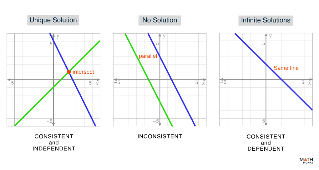
A system of linear equations normally has a single solution, but sometimes, it can have no solution or infinite solutions depending on the relationship between the equations. We can verify these solutions either algebraically or graphically:
Unique Solution (Consistent and Independent System)
A system is said to have a unique solution if it has exactly one solution. This occurs when the equations represent two lines that intersect at a single point.
For example, the system 2x + y = 5, x – y = 1 has the solution (2, 1)
No Solution (Inconsistent System)
A system has no solution if the equations represent parallel lines and thus can never intersect.
For example, the system 2x + y = 3, 4x + 2y = 8 has no solution
Infinite Solutions (Consistent and Dependent System)
A system has infinitely many solutions when a system of equations is represented by the same line, which means every point on the line is a solution.
For example, 2x + 4y = 8, x + 2y = 4 are identical, and thus the system has infinitely many solutions.
Solving
We use different methods to solve a system of linear equations. It depends on the complexity of the system and the way we want to solve it.
By Graphing
This method provides a visual way to find the solution. Each equation is plotted as a straight line on a coordinate plane. The point where the lines intersect represents the solution to the system.
Let us consider the system:
y = 2x + 1 …..(i)
y = -x + 4 …..(ii)
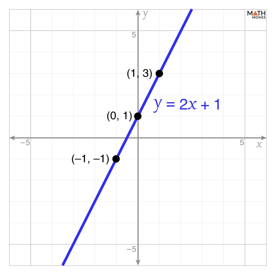
Step 1: Graphing the First Equation
From equation (i),
y = 2x + 1
Here, the slope m is 2, and the y-intercept c is 1
Thus, the coordinates of the y-intercept are (0, 1)
Now, using the slope and y-intercept, we get
x
2x + 1
y
-1
2(-1) + 1
-1
0
2(0) + 1
1
1
2(1) + 1
3
After plotting these points, we get
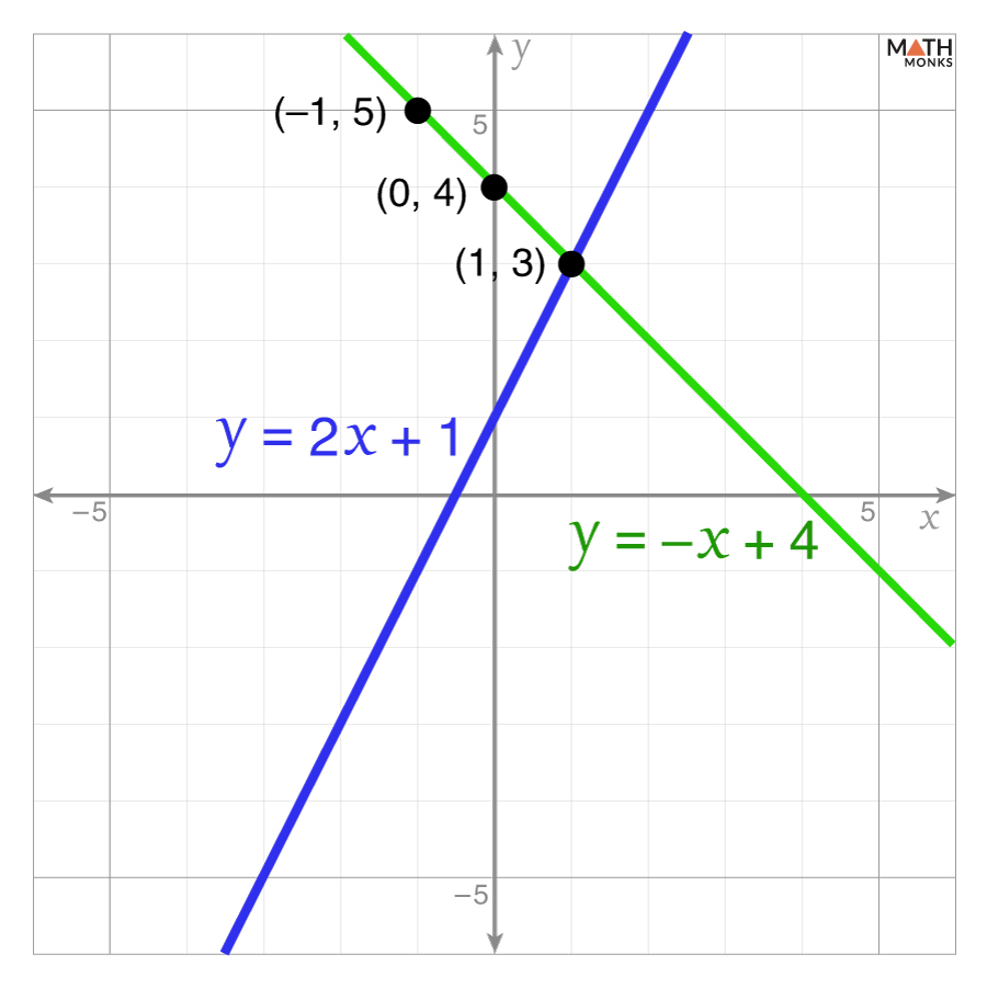
Step 2: Graphing the Second Equation
From equation (ii),
y = -x + 4
Here, the slope m is -1, and the y-intercept c is 4
Thus, the coordinates of the y-intercept are (0, 4)
Now, using the slope and y-intercept, we get
x
-x + 4
y
-1
-(-1) + 4
5
0
-(0) + 4
4
1
-(1) + 4
3
After plotting these points, we get
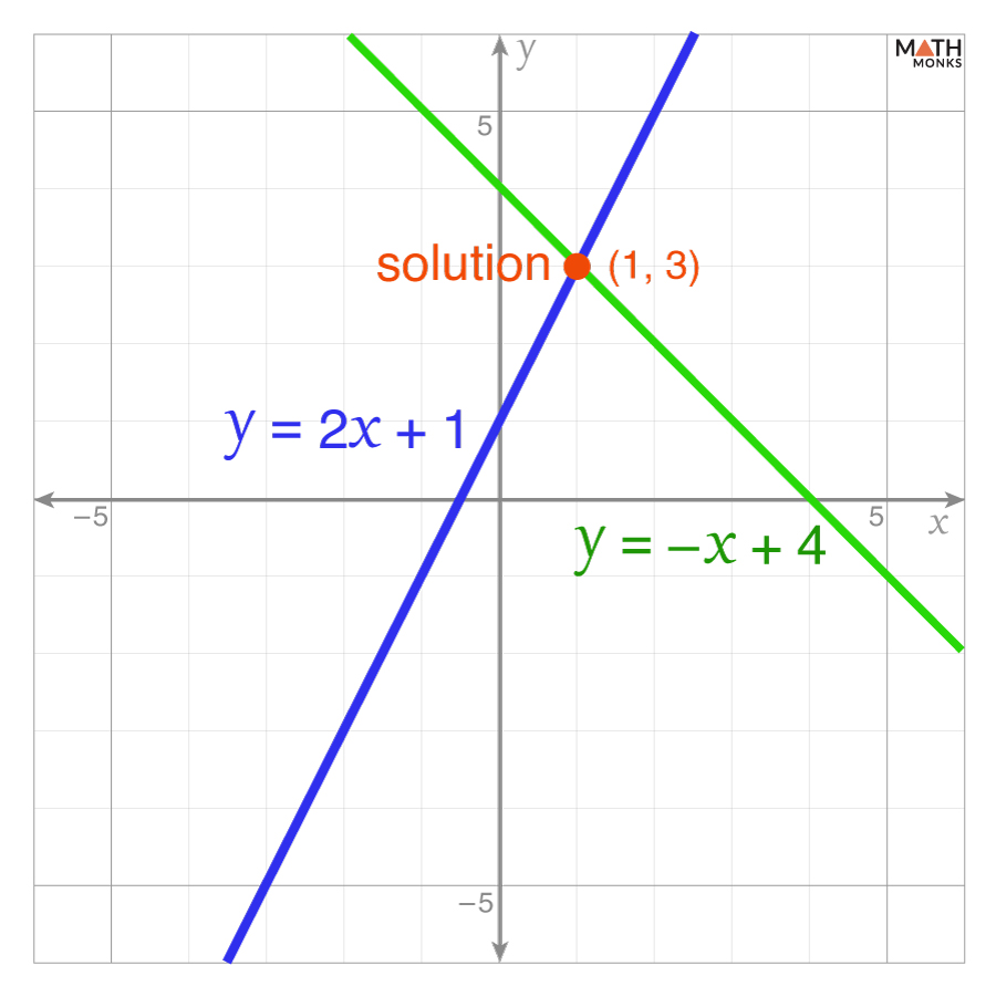
Step 3: Identifying the Intersection Point
Now, observing the graphs of these two lines, we conclude
The two lines intersect at (1, 3).
This means the solution to the system is x = 1 and y = 3
Here, since two lines intersect at one point (1, 3), the given system has one unique solution.
Note: Graphing may not always give accurate solutions, especially when working with decimals or fractions.
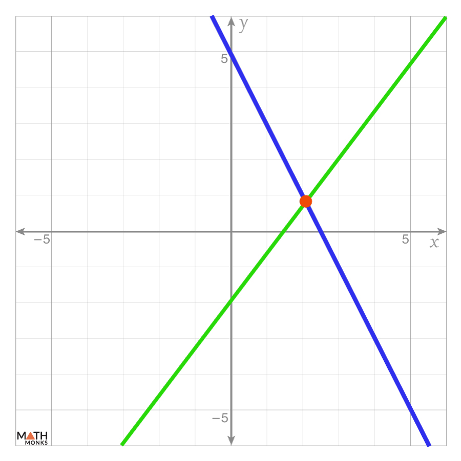
Determine the nature of the system:
Solution:
As we can observe, the lines have one intersection point on the graph. They have one unique solution. Thus, the system is consistent and independent.
By Substitution
In this method, we solve one equation for a variable in terms of the other and substitute it into the second equation. This transforms the system into a single equation with one variable which makes the system easier to solve. Once we find the value of the first variable, we substitute it back into the original equation to determine the second variable.
Let us consider the system:
x + y = 6 …..(i)
2x – y = 3 …..(ii)
Step 1: Solving for one variable in Terms of the Other
First, we solve for x in terms of y.
From equation (i),
x = 6 – y …..(iii)
Step 2: Substituting
Now, substituting (iii) into the equation (ii),
2(6 – y) – y = 3
⇒ 12 – 2y – y = 3
⇒ 12 – 3y = 3
⇒ 3y = 12 – 3
⇒ 3y = 9
⇒ y = 3
Step 3: Solving for x
Substituting y = 3 back into (iii), we get
x = 6 – 3
⇒ x = 3
Thus, the solution is x = 3 and y = 3
Solve the following linear equations by substitution: 2x + 3y = 18 4x + 2y = 22
This method involves adding or subtracting the given equations to eliminate one variable, simplifying the system into a single equation with one variable. Once we solve for that variable, we substitute its value back into one of the original equations to find the remaining variable(s).
Let us consider the system:
3x + 2y = 12 …..(i)
5x – 2y = 8 …..(ii)
Step 1: Adding the Equations
(3x + 2y) + (5x – 2y) = 12 + 8
⇒ 3x + 2y + 5x – 2y = 20
Step 2: Simplifying
⇒ 3x + 5x = 20
⇒ 8x = 20
⇒ x = ${\dfrac{20}{8}}$
⇒ x = ${\dfrac{5}{2}}$
Step 3: Substituting
Substituting x = ${\dfrac{5}{2}}$ back into equation (i), we get
⇒ ${3\left( \dfrac{5}{2}\right) +2y=12}$
⇒ ${\dfrac{15}{2}+2y=12}$
⇒ ${2y=12-\dfrac{15}{2}}$
⇒ ${2y=\dfrac{24-15}{2}}$
⇒ ${2y=\dfrac{9}{2}}$
⇒ ${y=\dfrac{9}{4}}$
Thus, the solution is x = ${\dfrac{5}{2}}$ and ${y=\dfrac{9}{4}}$
What is the solution to this system of linear equations? (Use elimination method) 4x + 3y = 20 2x – 3y = 4
The inverse matrix method is particularly useful for solving complex or larger systems of linear equations. In this approach, the system is rewritten in matrix form as:
AX = B
To solve the system, we find the matrix X, which represents the values of the unknowns.
Here,
A is the coefficient matrix containing the coefficients of the variables
X is the variable matrix representing the unknown variables
B is the constant matrix containing the constant terms from the right-hand side of the equations
The solution can be found using the formula:
X = A-1B
Note: Since A-1 exists, A is an invertible matrix.
Now, let us solve the system of linear equations:
2x + 3y = 8 …..(i)
4x + y = 5 …..(ii)
Step 1: Expressing the System in Matrix Form
To organize the equations in a standard way, we rewrite the equations (i) and (ii) in the matrix form as:
AX = B
⇒ ${\begin{bmatrix} 2 & 3 \\ 4 & 1 \end{bmatrix}\begin{bmatrix} x \\ y \end{bmatrix}=\begin{bmatrix} 8 \\ 5 \end{bmatrix}}$
Step 2: Finding the Inverse of Matrix A
To compute the inverse matrix of A, we first find the determinant A. If A is invertible (i.e., whether an inverse matrix exists):
If det(A) = 0, the system has no unique solution, which means the system may be inconsistent or have infinitely many solutions.
If det(A) ≠ 0, we proceed to the next step.
Now, for the given matrix A = ${\begin{bmatrix} 2 & 3 \\ 4 & 1 \end{bmatrix}}$,
⇒ ${\begin{bmatrix} x \\ y \end{bmatrix}=\begin{bmatrix} -0.1 & 0.3 \\ 0.4 & -0.2 \end{bmatrix}\begin{bmatrix} 8 \\ 5 \end{bmatrix}}$
Multiplying the matrices, we get
x = (-0.1 × 8) + (0.3 × 5) = -0.8 + 1.5 = 0.7
y = (0.4 × 8) + (-0.2 × 5) = 3.2 – 1 = 2.2
Thus, the solution to the system is x = 0.7 and y = 2.2
By Gaussian Elimination Method
The Gaussian elimination method is often used for larger systems with three or more equations. It involves converting the system into row echelon form and then using back-substitution to find the variable values.
Let us solve the system of equations:
2x + y – z = 8 …..(i)
-3x – y + 2z = -11 …..(ii)
-2x + y + 2z = -3 …..(iii)
Step 1: Converting the System of Equations into an Augmented Matrix
To organize the equations systematically, we express the system as an augmented matrix. It is a matrix where the column of constants is added to the right side of the coefficient matrix.
If we have the system in upper triangular form, we solve for variables starting from the last row,
From the last row,
z = -1
Substituting z = -1 into the second row,
2y + (-1) = 5
⇒ 2y = 6
⇒ y = 3
Substituting y = 3 and z = -1 into the first row,
2x + 3 – (-1) = 8
⇒ 2x + 4 = 8
⇒ x = 2
Thus, the solution is (x, y, z) = (2, 3, -1)
By Cramer’s Rule
This method is used when the system of equations has the same number of equations as unknowns, and the determinant of the coefficient matrix is nonzero.
To solve a system of n linear equations with n variables, we use the formula:
Thus, the solutions are: x = ${\dfrac{4}{7}}$ and y = ${\dfrac{9}{7}}$
Solve using the inverse matrix method: 2x + 3y = 8 4x – y = 2
Solution:
Given, 2x + 3y = 8 …..(i) 4x – y = 2 …..(ii) Step 1: Expressing the System in Matrix Form The given system can be written as: AX = B ⇒ ${\begin{bmatrix} 2 & 3 \\ 4 & -1 \end{bmatrix}\begin{bmatrix} x \\ y \end{bmatrix}=\begin{bmatrix} 8 \\ 2 \end{bmatrix}}$ Here, A = ${\begin{bmatrix} 2 & 3 \\ 4 & -1 \end{bmatrix}}$ X = ${\begin{bmatrix} x \\ y \end{bmatrix}}$ B = ${\begin{bmatrix} 8 \\ 2 \end{bmatrix}}$ Step 2: Finding the Inverse of Matrix A Calculating det(A), we get det(A) = (2)(-1) – (3)(4) = -2 – 12 = -14 Since det(A) ≠ 0, the inverse exists. Now, calculating A-1, we get ${A^{-1}=\dfrac{1}{\det \left( A\right) }\cdot adj\left( A\right)}$ ⇒ ${A^{-1}=\dfrac{1}{-14}\begin{bmatrix} 1 & -3 \\ -4 & 2 \end{bmatrix}=\begin{bmatrix} \dfrac{1}{14} & \dfrac{3}{14} \\ \dfrac{4}{14} & \dfrac{-2}{14} \end{bmatrix}}$ Step 3: Solving for X Since AX = B ⇒ X = A-1B ⇒ X = ${\begin{bmatrix} \dfrac{1}{14} & \dfrac{3}{14} \\ \dfrac{4}{14} & -\dfrac{2}{14} \end{bmatrix}\begin{bmatrix} 8 \\ 2 \end{bmatrix}}$ ⇒ X = ${\begin{bmatrix} \dfrac{1}{14}\times 8+\dfrac{3}{14}\times 2 \\ \dfrac{4}{14}\times 8-\dfrac{2}{14}\times 2 \end{bmatrix}}$ ⇒ X = ${\begin{bmatrix} \dfrac{14}{14} \\ \dfrac{28}{14} \end{bmatrix}}$ ⇒ X = ${\begin{bmatrix} 1 \\ 2 \end{bmatrix}}$ Thus, the solutions are: x = 1 and y = 2
 Determine the nature of the system: