Logarithmic Spiral

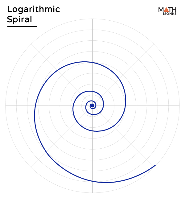
A logarithmic spiral, also called an equiangular spiral or growth spiral, is a special type of curve found in nature, such as spider webs, shells of some mollusks, and the fossils of ammonites. It cuts all radial lines at a constant angle θ.  

Descartes first described it, which was later explained by Jakob Bernoulli.

The logarithmic spiral relates to the golden rectangle, the golden ratio, and the fibonacci spiral, and thus, sometimes, it is referred to as the golden spiral. 

Equations

Polar Form

In polar coordinates (r, θ), the curve is written as:

r = ae^bθ

Here, 

r = the distance from the origin (radius)

θ = the angle in radians

a, b = arbitrary constants, determining the scale and the shape of the spiral

b = cotα, polar tangential angle

Parametric Form

In parametric form, it is expressed as:

x = r cosθ = a cosθ e^bθ = a cosθ e^{θ cotα}

y = r sinθ = a sinθ e^bθ = a sinθ e^{θ cotα}

Here, the rate of change of radius is 

${\dfrac{dr}{d\theta }=abe^{b\theta }=br}$ 

The angle between the tangent and the radial line at the point (r, θ) is 

${\alpha =\tan ^{-1}\left( \dfrac{r}{\dfrac{dr}{d\theta }}\right) =\tan ^{-1}\left( \dfrac{1}{b}\right) =\cot ^{-1}b}$

Since b → 0 and α → ${\dfrac{\pi }{2}}$, the spiral converges towards a circle.

Example

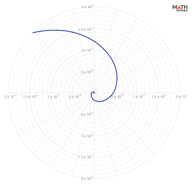
Let us consider a logarithmic spiral whose a = 7.5 and α = 1 radian

Here, r = 7.5 e^{θ cot(1)}, whose equiangular graph is as shown.

Here, any radius vector forms the same angle in the curve, and thus, the curve is equiangular.

Geometric Sequence

Whenever a point is located in the logarithmic spiral, its length is finite from the radius to the origin. A radius vector measures the distance from the origin to the point, while arc length measures the distance from the point to the pole. 

The logarithmic spiral follows a pattern that meets at a geometrically progressive distance from the origin.

Arc Length

The given formula finds the arc length of the logarithmic spiral:

${s=\int ds=\int \sqrt{\left( x’\right) ^{2}+\left( y\right) ^{2}}dt=\dfrac{a\sqrt{1+b^{2}}}{b}e^{b\theta }}$

⇒ ${s=\dfrac{r\sqrt{1+b^{2}}}{b}}$

Curvature

The curvature of the logarithmic spiral is calculated using the formula:

${k=\dfrac{x’y”-y’x”}{\left( \left( x’\right) ^{2}+\left( y’\right) ^{2}\right)^{\dfrac{3}{2}}}}$

⇒ ${k=\dfrac{e^{-b\theta }}{a\sqrt{1+b^{2}}}}$

Tangential Angle

The given formula determines the tangential angle of the logarithmic spiral:

${\phi =\int k\left( s\right) ds=\theta}$

Inversion

The inversion of the logarithmic spiral with respect to its center yields a spiral that is equal dimensionally. The inversion maps the spiral of r = ae^bθ onto another logarithmic spiral, which is ${r=\dfrac{1}{a}e^{-b\theta }}$

Pedal

The given formulas find the pedal curve of the logarithmic spiral in the parametric form:

f = e^aα cosα, g = e^aα sinα

At the pole, the pedal curve is an identical logarithmic spiral for a pedal point.

The pedal equation of the logarithmic spiral is:

${x=\dfrac{\left( a\sin \alpha +\cos \alpha \right) e^{a\alpha }}{1+a^{2}}}$

${y=\dfrac{\left( \sin \alpha -a\cos \alpha \right) }{1+a^{2}}e^{a\alpha }}$

Thus, r = ${\sqrt{x^{2}+y^{2}}=\dfrac{e^{a\alpha }}{\sqrt{1+a^{2}}}}$

Cartesian Equation

The cartesian equation of the logarithmic spiral is given by:

x² + y² = (a e^bθ)²

Cesàro Equation

The Cesàro Equation of the logarithmic spiral is written as:

${sk=\dfrac{1-ak\sqrt{1+b^{2}}}{b}}$

Antennas

The logarithmic spiral antennas are frequency-independent antennas whose polarization, radiation pattern, and impedance remain largely unmodified over a wide range.