Intermediate Value Theorem

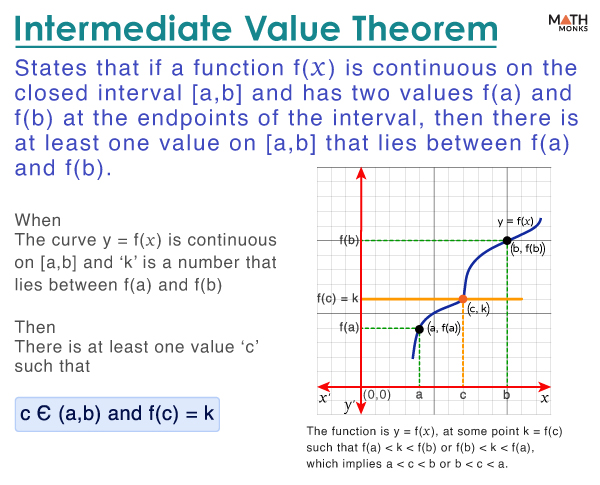
The intermediate value theorem (IVT) is about continuous functions in calculus. It states that if a function f(x) is continuous on the closed interval [a, b] and has two values f(a) and f(b) at the endpoints of the interval, then there is at least one value on [a, b] that lies between f(a) and f(b).

Formula

Mathematically, the IVT is written as:

When

• The curve y = f(x) is continuous on [a, b]
• ‘k’ is a number that lies between f(a) and f(b)

Then, 

• There is at least one value ‘c’ such that c Є (a, b) and f(c) = k

Thus, the function y = f(x) at some point k = f(c) where either f(a) < k < f(b) or f(b) < k < f(a), which means a < c < b or b < c < a.

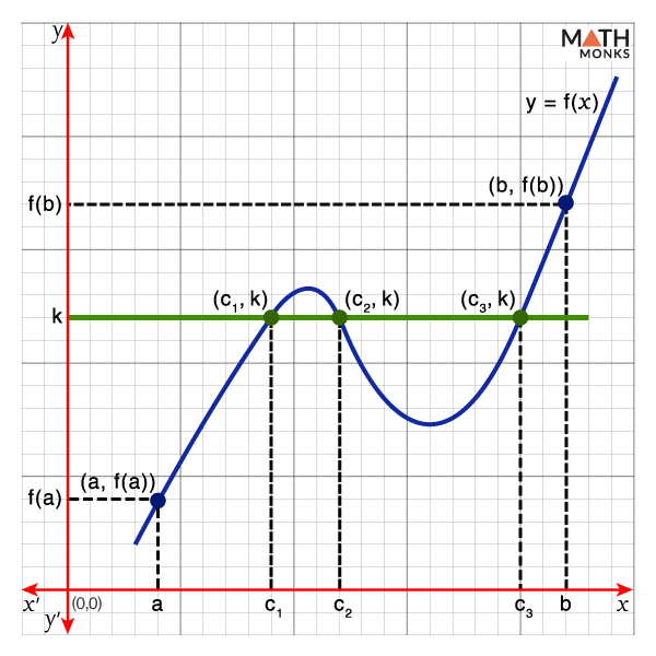
Here, the graph of y = f(x) is drawn in a continuous way within the interval [a, b], and thus, f(x) is continuous on [a, b]. In addition, if a value ‘c’ exists within the interval [a, b] such that c Є (a, b), then f(c) = k and f(a) < f(c) < f(b).

Since there exists ‘at least one value’ within the given interval, there can be more.

For example, there are three points where f(x) = k, as shown.

In the graph, f(c₁) = f(c₂) = f(c₃) = k, which means there are three values ‘c₁,’ ‘c₂,’ and ‘c₃’ on [a, b] with the function value ‘k.’

In particular, when c = 0, the intermediate value theorem is called Bolzano’s theorem (after its discoverer, Bernard Bolzano) or the Intermediate Zero Theorem.

Proof

To prove the IVT, we use the limit definition.

Without loss of generality, let us assume that f(a) < k < f(b) and a set A = {x Є [a, b]: f(x) < k}

Here, the set ‘A’ is non-empty since a Є A and f(a) < k, and also, ‘A’ is bounded above by ‘b.’

Thus, by completeness property, it has a supremum, say ‘c,’ which is greater than or equal to each element of ‘A’ and f(c) = k.

Proving c Є (a, b)

Since the function f(x) is continuous at ‘a’ and ‘b,’ f(c) ≠ a and f(c) ≠ b and thus c Є (a, b)

Proving f(c) = k

To prove f(c) = k, we verify both f(c) ≤ k and f(c) ≥ k.

Proving f(c) ≤ k

Since ‘c’ is the supremum, from the extreme value theorem, we get a sequence x_n Є A where x_n → c

Since f(x) is continuous, so f(x_n) → f(c)

Again, since x_n Є A, by definition of ‘A,’ f(x_n) < k

⇒ f(c) = ${\lim _{n\rightarrow \infty }f\left( x_{n}\right) \leq k}$

Thus, f(c) ≤ k is proved …..(i)

Proving f(c) ≥ k:

Since c < b, thus for a very small ‘n,’ t_n = ${c+\dfrac{1}{n} <b}$

⇒ t_n > c 

⇒ t_n > supremum of ‘A’

⇒ t_n ∉ A

Thus, f(t_n) ≥ k

Since ‘n’ is considered to be very small and f(x) is continuous, so f(t_n) → f(c), which implies

f(c) = ${\lim _{n\rightarrow \infty }f\left( t_{n}\right) \geq k}$

Thus, f(c) ≥ k is proved …..(ii)

From (i) and (ii), we conclude that f(c) = k

Thus, the intermediate value theorem is proved.

How to Use

Verifying the Roots in an Interval

The intermediate value theorem is used to verify the existence of an equation’s root in a given interval, which shows whether the given function has its zero (or f(x) = 0) within the interval (a, b). 

Let us verify this statement using the function f(x) = x⁴ – 2x³ + 3x – 21, which has a zero within the interval [1, 3]

Step 1: Finding f(a) and f(b)

Here, the given interval is [1, 3]

Calculating f(1) and f(3), we get

At x = 1, f(1) = (1)⁴ – 2(1)³ + 3(1) – 21 = -19

At x = 3, f(3) = (3)⁴ – 2(3)³ + 3(3) – 21 = 15

Step 2: Verifying

Since f(1) is negative, the curve is below zero at x = 1. Similarly, since f(3) is positive, the curve is above zero at x = 3.

Also, as f(x) is a polynomial function, it is continuous.

Now, by the intermediate value theorem, we conclude that the curve must pass through some point ‘c’ (say) within [1, 3] such that f(c) = 0

Hence, there exists a solution to the function f(x) = x⁴ – 2x³ + 3x – 21 on [1, 3] such that f(x) = 0

Limitations

However, we can only verify whether the function has a root in the given interval using the intermediate value theorem. We cannot find the number of roots or their values from it. 

Considering the previous example, f(x) = x⁴ – 2x³ + 3x – 21, which has some root ‘c’ within [1, 3] such that f(c) = 0.

Thus, from the intermediate value theorem, the function f(x) = x⁴ – 2x³ + 3x – 21 has some roots, but the number of roots and their values cannot be obtained.  

In addition to its theoretical applications, the intermediate value theorem has many real-life applications. One of them, ‘The Mystery of the Wobbly Table,’ is discussed. 

Fixing a Wobbly Table

The intermediate value theorem helps to fix a wobbly table. 

Here is an example of uneven ground causing a wobbly table. If the ground is continuous, and poorly fitted tiles cause no ups and downs, we rotate the table to fix the problem.

In a wobbly table, where three legs touch the ground, and the fourth leg is disturbed due to poorly fitted tiles, we can solve the issue using the intermediate value theorem. According to the theorem, there is a point where the fourth leg touches the ground perfectly. Finding the point will help us fix the issue.

It is based on the assumption that if we rotate a table and the 4^th leg goes inside the ground, then at some point, it will be above the ground, and at another point, it will be below the ground.

Mean Value Theorem vs. Intermediate Value Theorem  

• The mean value theorem applies to differentiable functions and their derivatives, whereas the intermediate theorem applies to continuous functions.
• The mean value theorem guarantees the derivatives with certain values, whereas the intermediate value theorem confirms that the function has certain values between two given points within the interval.

Solved Example