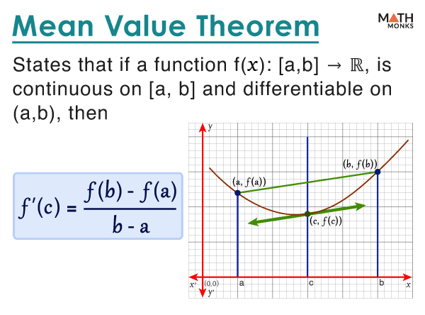
The mean value theorem (MVT) or Lagrange’s mean value theorem (LMVT) states that if a function ‘f’ is continuous on the closed interval [a, b] and differentiable on the open interval (a, b), then there exists a point c Є (a, b) such that the tangent through ‘c’ is parallel to the secant passing through the endpoints of the curve.
${f’\left( c\right) =\dfrac{f\left( b\right) -f\left( a\right) }{b-a}}$
Mathematically,
If f(x): [a, b] → ℝ, is continuous on [a, b] and differentiable on (a, b), then
${f’\left( c\right) =\dfrac{f\left( b\right) -f\left( a\right) }{b-a}}$, where c Є (a, b)
Applications of the mean value theorem are found in mathematical analysis, computational mathematics, and many other fields.
Graphing
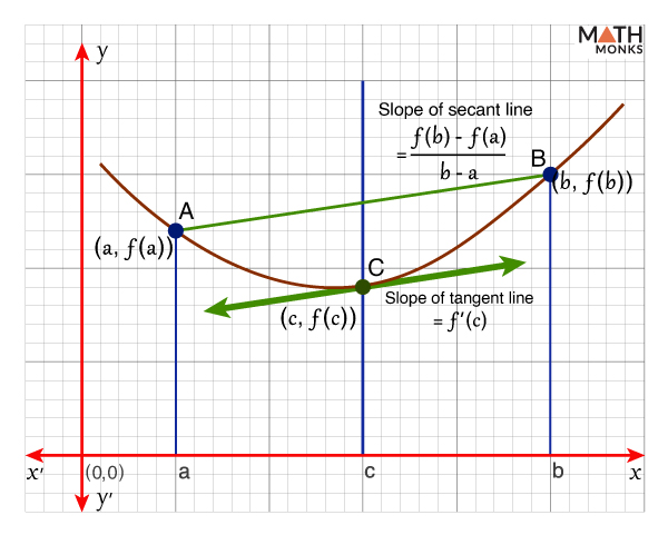
To represent visually, let us graph the equation y = f(x).
The graph of y = f(x) passes through the points A (a, f(a)) and B (b, f(b)), as shown.
Here, the derivative at C gives the slope of the tangent for f(x) at x = c, which means there exists a point between A and B, and the slope of the tangent equals the slope of the line joining the points at x = a and x = b.
Thus, the tangent at point ‘c’ is parallel to the secant AB.
Proof
Let g(x) be a secant to f(x), passes through the points (a, f(a)) and (b, f(b)).
Now, the slope of the secant is ${m =\dfrac{f\left( b\right) -f\left( a\right) }{b-a}}$ and the equation of the secant is y – y1 = m(x – x1)
⇒ ${y-f\left( a\right) =\dfrac{f\left( b\right) -f\left( a\right) }{b-a}\times \left( x-a\right)}$
⇒ ${y=\dfrac{f\left( b\right) -f\left( a\right) }{b-a}\times \left( x-a\right) +f\left( a\right)}$
Considering the equation of the secant as g(x) = y, we get
${g\left( x\right) =\dfrac{f\left( b\right) -f\left( a\right) }{b-a}\times \left( x-a\right) +f\left( a\right)}$…..(i)
Now, let us define a function, h(x) = f(x) – g(x)
from (i), ${h\left( x\right) =f\left( x\right) -\left[ \dfrac{f\left( b\right) -f\left( a\right) }{b-a}\left( x-a\right) +f\left( a\right) \right]}$
If h(x) is continuous on [a,b] and differentiable on (a,b).
By applying Rolle’s theorem (a special case of the mean value theorem), we get
h'(c) = 0 for c Є (a, b), and ${h’\left( x\right) =f’\left( x\right) -\dfrac{f\left( b\right) -f\left( a\right) }{b-a}}$
Now, for some c Є (a, b), h'(c) = 0
⇒ ${f’\left( c\right) -\dfrac{f\left( b\right) -f\left( a\right) }{b-a}}$ = 0
⇒ ${f’\left( c\right) =\dfrac{f\left( b\right) -f\left( a\right) }{b-a}}$
Thus, the mean value theorem is proved.
Alternate Method
Let us consider the auxiliary function F(x) = f(x) + px
We choose a number p that satisfies the condition F(a) = F(b)
f(a) + pa = f(b) + pb
⇒ f(b) – f(a) = p(a – b)
⇒ p = ${-\dfrac{f\left( b\right) -f\left( a\right) }{b-a}}$
Thus, ${F\left( x\right) =f\left( x\right) -\dfrac{f\left( b\right) -f\left( a\right) }{b-a}x}$
Here, F(x) is continuous on [a, b] and differentiable on (a, b), and F(a) = F(b), which satisfies all the conditions of Rolle’s theorem.
Thus, a point ‘c’ exists on (a, b), where F’(c) = 0
⇒ ${f’\left( c\right) -\dfrac{f\left( b\right) -f\left( a\right) }{b-a}}$ = 0
⇒ ${f’\left( c\right) =\dfrac{f\left( b\right) -f\left( a\right) }{b-a}}$, proven.
Since there can be any number of points on (a, b), Lagrange’s Mean Value Theorem is also called the finite mean value theorem.
Now, let us apply Langrange’s mean value theorem to the function f(x) = 3x2 – 10x + 5 on [0, 3].
Since f(x) is a polynomial function, it is continuous on [0, 3] and differentiable (0, 3), which satisfies the conditions of the MVT.
Now, f(0) = 3(0)2 – 10(0) + 5 = 5
f(3) = 3(3)2 – 10(3) + 5 = 2
By MVT, there exists a point c Є (0, 3), f’(c) = 6c – 10
Also, ${f’\left( c\right) =\dfrac{f\left( b\right) -f\left( a\right) }{b-a}}$
⇒ ${6c-10=\dfrac{2-5}{3-0}}$
⇒ ${6c-10=\dfrac{-3}{3}}$
⇒ ${6c=-1+10}$
⇒ ${c=\dfrac{9}{6}}$
⇒ ${c=\dfrac{3}{2}}$ Є (0, 3)
Thus, the mean value theorem is verified.
Interpretation
If f(t) represents the position of an object moving along a line, with respect to the time ‘t,’ then the average velocity of the body for the period b – a is ${\dfrac{f\left( b\right) -f\left( a\right) }{b-a}}$.
Here, the mean value theorem explains the average change in function on [a, b], whereas f'(c) represents the instantaneous change at ‘c.’
According to MVT, the average change in the function f(x) on [a, b] equals the instantaneous change f'(x) at point c for c Є (a, b).
Let us suppose a car moving along a straight line for 1 hour with an average velocity of 60 mph. Here, 0 ≤ t ≤ 1 hour, s(t) = the position of the car and v(t) = the velocity of the car.
Now, assuming that the position function s(t) is differentiable and applying the MVT, we get:
At some time c Є (0, 1), the speed of the car is exactly = v(c) = s′(c) = ${\dfrac{s\left( 1\right) -s\left( 0\right) }{1-0}}$ = 60 mph.
Solved Example
![]() Verify the mean value theorem for ${f\left( x\right) =\sqrt{x+1}}$ on [-1, 0]
Verify the mean value theorem for ${f\left( x\right) =\sqrt{x+1}}$ on [-1, 0]
Solution:
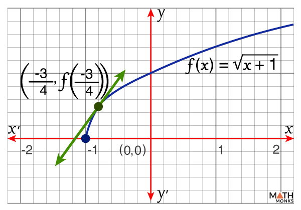
As we know, f(x) is continuous on [-1, 0] and differentiable (-1, 0), which satisfies the conditions of the MVT.
Now, ${f\left( -1\right) =\sqrt{-1+1}}$ = 0
${f\left( 0\right) =\sqrt{0+1}}$ = 1
By MVT, there exists a point c Є (-1, 0), ${f’\left( c\right) =\dfrac{1}{2\sqrt{c+1}}}$
Also, ${f’\left( c\right) =\dfrac{f\left( b\right) -f\left( a\right) }{b-a}}$
⇒ ${\dfrac{1}{2\sqrt{c+1}}=\dfrac{f\left( 0\right) -f\left( -1\right) }{0+1}}$
⇒ ${\dfrac{1}{2\sqrt{c+1}}=\dfrac{1-0}{1}}$
⇒ ${2\sqrt{c+1}=1}$
⇒ ${\sqrt{c+1}=\dfrac{1}{2}}$
⇒ ${c+1=\dfrac{1}{4}}$
⇒ ${c=-\dfrac{3}{4}}$ Є (-1, 0)
Thus, the mean value theorem is verified and ${c=-\dfrac{3}{4}}$
Corollaries
As we know, the derivative of any constant function is 0. The Mean Value Theorem allows that the converse is also true, which means, ∀ x at some interval I, if the derivative,f′(x) = 0, f(x) is constant over that interval.
Corollary 1.
Let ‘f’ be differentiable at an interval ‘I.’ If f′(x) = 0, ∀ x Є I, then f(x) is constant, ∀ x Є I.
Proof: Since ‘f’ is differentiable on ‘I,’ ‘f’ is continuous over ‘I.’
Let us consider that f(x) is not constant, ∀ x in I. Then there exists a, b Є I, where a ≠ b and f(a) ≠ f(b).
Now, for a < b, we get ${\dfrac{f\left( b\right) -f\left( a\right) }{b-a}}$ ≠ 0.
Since f is differentiable, by MVT, there exists c Є (a,b) such that f′(c) = ${\dfrac{f\left( b\right) -f\left( a\right) }{b-a}}$
Thus, c Є I exists such that f‘(c) ≠ 0, which contradicts the assumption f′(x) = 0, ∀ x Є I.
Thus, according to Corollary 1, if two functions have the same derivative, they differ by at most one constant.
Corollary 2.
If 2 functions, ‘f’ and ‘g,’ are differentiable on an interval I and f′(x) = g′(x), ∀ x Є I, then f(x) = g(x) + C, for some constant C.
Proof: Let us define, h(x) = f(x) – g(x)
Since the two functions f(x) and g(x) are continuous on [a, b] and differentiable on (a, b), h(x) is also continuous and differentiable.
Thus, h′(x) = f′(x) – g′(x)
However, by assumption f′(x) = g’(x), ∀ x on (a,b), we have h′(x) = 0, ∀ x on (a,b).
Thus, by Corollary 1, h(x) is constant on the interval.
This means that we have h(x) = c
⇒ f(x) – g(x) = c
⇒ f(x) = g(x) + c, proven.
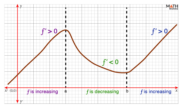
Thus, MVT shows that if a function’s derivative is positive, the function is increasing. Conversely, if the derivative is negative, the function is decreasing.
Corollary 3.
Let ‘f’ be continuous on [a, b] and differentiable on (a, b).
- If f’(x) > 0, ∀ x Є (a, b), then ‘f’ is an increasing function on [a, b].
- If f’(x) < 0, ∀ x Є (a, b), then ‘f’ is a decreasing function on [a, b].
Proof for 1
Let us consider that ‘f’ is not an increasing function on an interval ‘I,’ then there exists ‘a,’ b Є I such that a < b, but f(a) ≥ f(b).
Since f is differentiable on I, by MVT, there exists c Є (a, b) such that ${f’\left( c\right) =\dfrac{f\left( b\right) -f\left( a\right) }{b-a}}$
Now, f(a) ≥ f(b)
⇒ f(b) – f(a) ≤ 0
Also, a < b
⇒ b – a > 0
Thus, ${f’\left( c\right) =\dfrac{f\left( b\right) -f\left( a\right) }{b-a}}$ ≤ 0
However, f’(x) > 0 is a contradiction since ‘f’ is an increasing function on ‘I.’
Proof for 2
Let us consider that ‘f’ is not a decreasing function on an interval ‘I,’ then there exists a, b Є I such that a < b, and f(a) ≤ f(b).
Since f is differentiable on I, by MVT, there exists c Є (a, b) such that ${f’\left( c\right) =\dfrac{f\left( b\right) -f\left( a\right) }{b-a}}$
Now, f(a) ≤ f(b)
⇒ f(b) – f(a) ≥ 0
Also, a < b
⇒ b – a > 0
Thus, ${f’\left( c\right) =\dfrac{f\left( b\right) -f\left( a\right) }{b-a}}$ ≥ 0
However, f’(x) < 0 is a contradiction since ‘f’ is a decreasing function on ‘I.’