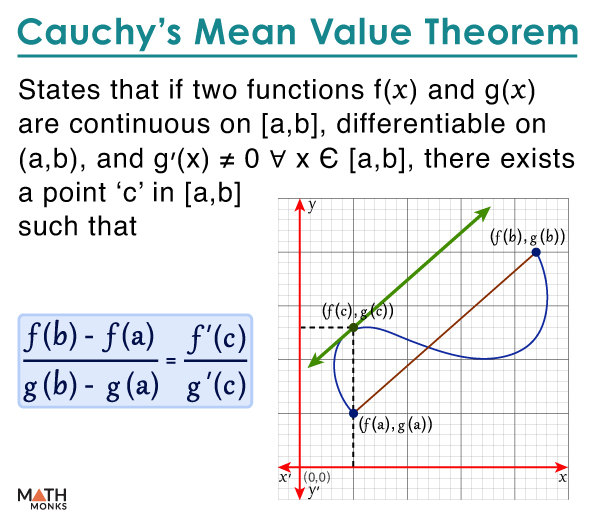
Cauchy’s Mean Value Theorem

Cauchy’s mean value theorem states that if two functions, f(x) and g(x), are continuous on the closed interval [a, b] and differentiable on the open interval (a, b), then there exists a point ‘c’ on [a, b] such that ${\dfrac{f\left( b\right) -f\left( a\right) }{g\left( b\right) -g\left( a\right) }=\dfrac{f’\left( c\right) }{g’\left( c\right) }}$

It is thus a generalization of the mean value theorem or Lagrange’s mean value theorem.

Cauchy’s mean value theorem, also called the extended or second mean value theorem, establishes the relationship between the derivatives of two functions and their changes at a given interval.

Mathematically, 

If 2 functions f(x) and g(x) are continuous on [a, b], differentiable on (a, b), and g’(x) ≠ 0 ∀ x Є [a, b], then

a point c Є [a, b] exists such that ${\dfrac{f\left( b\right) -f\left( a\right) }{g\left( b\right) -g\left( a\right) }=\dfrac{f’\left( c\right) }{g’\left( c\right) }}$

Proof

Let f(x) and g(x) be the functions, continuous on [a, b] and differentiable on (a, b).

Also, g’(x) ≠ 0 ∀ x Є [a, b]

Now, let us consider an auxiliary function F(x) such that 

F(x) = f(x) + m × g(x)…..(i), where m is chosen in such a way that F(a) = F(b)

Thus, f(a) + m × g(a) = f(b) + m × g(b)

⇒ f(b) – f(a) = m × [g(a) – g(b)]

⇒ m = ${-\dfrac{f\left( b\right) -f\left( a\right) }{g\left( b\right) -g\left( a\right) }}$

From (i), we get ${F\left( x\right) =f\left( x\right) -\dfrac{f\left( b\right) -f\left( a\right) }{g\left( b\right) -g\left( a\right) }g\left( x\right)}$, which is continuous on [a, b] and differentiable on (a, b) and F(a) = F(b)

Thus, by Rolle’s theorem, we have a point ‘c’ on [a, b] such that F’(c) = 0

⇒ ${f’\left( c\right) -\dfrac{f\left( b\right) -f\left( a\right) }{g\left( b\right) -g\left( a\right) }g\left( c\right) =0}$

⇒ ${\dfrac{f\left( b\right) -f\left( a\right) }{g\left( b\right) -g\left( a\right) }=\dfrac{f’\left( c\right) }{g’\left( c\right) }}$ the Cauchy mean value theorem is proven.

By putting g(x) = x in the above formula, we get

${\dfrac{f\left( b\right) -f\left( a\right) }{b-a}=f’\left( c\right)}$, which is the Lagrange’s mean value formula.

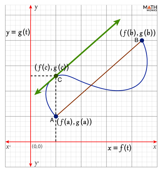
Now, let us make a graph using the parametric equations x = f(t) and y = g(t), where the parameter ‘t’ changes within the interval [a, b]. On changing the parameter, the point ‘C’ on the curve extends from A (f(a), g(a)) to B (f(b), g(b)), as shown.

Now, by Cauchy’s mean value theorem, the point C (f(c), g(c)) exists on the curve formed by the equations x = f(t) and y = g(t), where the tangent line is parallel to the chord AB joining the ends A and B of the curve.

Thus, Cauchy’s mean value theorem is proved.

Solved Examples